Pearson Correlation Analysis

Correlation Analysis

The linear correlation coefficient is a measure of the linear relationship between two random variables X and Y, denoted by r. So, r will measure the extent to which points are clustered around a straight line. If clustering points follow a straight line with a positive slope, then there is a high positive correlation between the two variables. Conversely, if the slope is negative, then there is a high negative correlation.

A positive correlation can be interpreted that for large X values ​​it will correspond to large Y values, or for small X values ​​it will match a small Y value too. Whereas a negative correlation occurs when large X values ​​will match small Y values ​​or vice versa. A perfect linear relationship will occur if r = +1 or -1 is obtained. If r approaches +1 or -1, the relationship between the two variables is strong and we say there is a high correlation between the two. But if r = 0 is obtained, then this implies that the absence of a linear relationship, does not mean that between the two variables there is no relationship. For the level of the relationship between the two variables whether it is very strong, strong or weak can be in the following table,

Correlation Value Interval	Explanation
0,00 – 0,199	Very Weak
0,20 – 0,399	Weak
0,40 – 0,599	Medium
0,60 – 0,799	Strong
0,80 – 1,000	Very Strong

Data exploration

Before doing a correlation analysis between variables, we should explore the data graphically first. Often we see patterns of relationships between variables by plotting the sample pairs of data on a cartesian diagram called a scatterplot or scatter diagram. Each data pair (x, y) is plotted as a single point.

Examples of scatter diagrams can be seen in the following figure.

Look and see, Graph a, b, c, it can be seen that the increase in y value is in line with the increase in the value of x. If the value of x increases, then the y value increases, and vice versa. From Graphs a to c, the distribution of data pair points is getting closer to a straight line which shows that the closeness of the relationship between x and y variables is getting stronger (synergistic).

The opposite happens in Graphs d, e, and f. Increasing the value of y is not in line with the increase in the value of x (antagonist). Increasing one value causes a decrease in the value of the partner. Once again it appears that the strength of the relationship between the two variables from d to f is getting stronger.

very contrary to the previous graph, in Graph g does not show a pattern of linear relationships between the two variables. This indicates that there is no correlation between the two variables. Finally, in Graph h we can see the pattern of relations between the two variables, only the pattern is not in the form of a linear relationship, but in a quadratic form.

Covariance and Correlation

To understand linear correlation between two variables, there are two elements that we must review, measuring the relationship between two variables (covariance) and the standardization process.

Covariance

One measure of the strength of the linear relationship between two continuous random variables is to calculate how much the two variables are covary, i.e. varying together. If one variable increases (or decreases) as a result of increasing (or decreasing) the pair variable, then the two variables are called covary. But if one variable does not change with increasing (or decreasing) other variables, then the variable is not covary. Statistics to measure how much of the two covary variables in the observation sample are covarians.

Besides, measuring how strong the relationship is between two variables, covariance also determines the direction of the relationship between the two variables.

1. If the value obtained is positive, it means that if the value of x is above the average value, then the value of y is also above the average value of y, and vice versa (Unidirectional).
2. The negative covariance value indicates that if the value of x is above the average value while the y value is below the average value (opposite direction).
3. Finally, if the covariance value is close to zero, it indicates that the two variables are not interconnected.

Standardization

One disadvantage of covariance as a measure of the strength of a linear relationship is the direction / strength of a gradient that depends on the units of the two variables. For example, the covariance between N uptake (%) and Animal Husbandry Results (tons) will be much greater if we convert% (1/100) to ppm (1 / million). If a covariant value is needed that does not depend on the unit of each variable, then we must standardize it first by dividing the covariance value by the standard deviation value of the two variables so that the value will be between -1 and +1. The statistical measure is known as the Pearson product moment correlation which measures the strength of the linear relationship (straight line) of the two variables. Linear correlation coefficients are sometimes referred to as Pearson correlation coefficients in honor of Karl Pearson (1857-1936), who first developed this statistical measure.

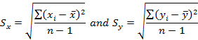
Standard Deviation of variables X and Y:

Correlation:

Covariance values ​​are standardized by dividing the covariance value by the standard deviation value of the two variables.

Correlation characteristics:

• The value of r always lies between the digits of -1 and +1
• The value of r does not change if all data is good at variable x, variable y, or both multiplied by a value of a constant (c) specified (provided c ≠ 0).
• The value of r does not change if all data is good at the x variable, y variable, or both added with a certain constant value (c).
• The value of r will not be affected by determining which variable x and which variable y. Both variables are interchangeable.
• The r value is only for measuring the strength of linear relationships, and is not designed to measure non-linear relationships

Assumption for correlation analysis:

Paired data samples (x, y) are random samples and quantitative data.

Samples Data (x, y) must be normally distributed.

Note: It must be remembered that correlation analysis is very sensitive to outliers!

Assumptions can be checked visually using:

Boxplots, histograms & univariate scatterplots for each variable

Bivariate scatterplots

If it does not fulfill one of the assumptions, for example, the data is not normally distributed (or there are data outliers), we can test it using Spearman correlation (Spearman rank correlation), correlation for non-parametric analysis.

Coefficient of Determination

The correlation coefficient, r, only provides a measure of strength and direction of a linear relationship between two variables. However, it does not provide information on what proportion of variation (variation) of the dependent variable (Y) can be explained or caused by a linear relationship with the value of the independent variable (X). The value of r cannot be compared directly, for example we cannot say that the value r = 0.8 is double the value of r = 0.4.

Fortunately, the square value of r can accurately measure the ratio / proposition, and this statistical value is called the Determination Coefficient, r². Thus, the Determination Coefficient can be defined as a value that states the diversity proportion Y which can be explained / explained by a linear relationship between variables X and Y.

For example, if the correlation value (r) between N uptake and yield = 0.8, then r² = 0.8 x 0.8 = 0.64 = 64%. This means that 64% of the diversity of rice yields can be explained / explained by the high and low uptake of N. The remaining 36% may be due to other factors or errors from the experiment.

SUBSCRIBE TO OUR NEWSLETTER

Share this post